Salience Maps for Text

Explore this demo yourself.

Or, run your own with examples/glue_demo.py

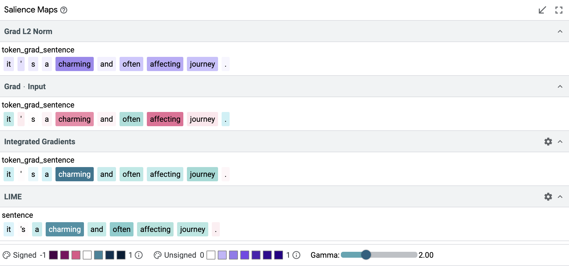
LIT enables users to analyze individual predictions for text input using salience maps, for which gradient-based and/or blackbox methods are available. In this tutorial, we will explore how to use salience maps to analyze a text classifier in the Classification and Regression models demo from the LIT website, and how these findings can support counterfactual analysis using LIT's generators, such as Hotflip, to test hypotheses. The Salience Maps module can be found under the Explanations tab in the bottom half of this demo and it supports four different methods for the GLUE model under test (with other models it might support a different number of these methods) - Grad L2 Norm, Grad · Input, Integrated Gradients (IG) and LIME.

Heuristics: Which salience method for which task?

Salience methods are imperfect. Research has shown that salience methods are often “sensitive to factors that do not contribute to a model's prediction”; that people tend to overly trust salience values or use methods they believe they know incorrectly; and that model architecture may directly impact the utility of different salience methods.

With those limitations in mind, the question remains as to which methods should be used and when. To offer some guidance, we have come up with the following decision aid that provides some ideas about which salience method(s) might be appropriate.

This flow chart can help you decide which salience interpreter to apply given the information provided by your model.

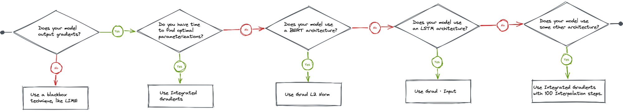
If your model does not output gradients with its predictions (i.e., is a blackbox), LIME is your only choice as it is currently the only black-box method LIT supports for text data.

If your model does output gradients, then you can choose among three methods: Grad L2 Norm, Grad · Input, and Integrated Gradients (IG). Grad L2 Norm and Grad · Input are easy to use and fast to compute, but can suffer from gradient saturation. IG addresses the gradient saturation issue in the Grad methods (described in detail below), but requires that the model output both gradients and embeddings, is much more expensive to compute, and requires parameterization to optimize results.

Remember that a good investigative process will check for commonalities and patterns across salience values from multiple salience methods. Further, salience methods should be an entry point for developing hypotheses about your model's behavior, and for identifying subsets of examples and/or creating counterfactual examples that test those hypotheses.

Salience Maps for Text: Theoretical background and LIT overview

All methods calculate salience, but there are subtle differences in their approaches towards calculating a salience score for each token. Grad L2 Norm only produces absolute salience scores while other methods like Grad · Input (and also Integrated Gradients and LIME) produce signed values, leading to an improved interpretation of whether a token has positive or negative influence on the prediction.

LIT uses different color scales to represent signed and unsigned salience scores. Methods that produce unsigned salience values, such as Grad L2 Norm, use a purple scale where darker colors indicate greater salience, whereas the other methods use a red-to-green scale, with red denoting negative scores and green denoting positive.

The tokens from same example in the SST-2 dataset can have dramatically different scores depending on the interpreter, as seen in this screenshot. Different salience interpreters output scores in different ranges, for example, Grad L2 Norm outputs unsigned values in the range from 0 to 1, denoted by the purple colors (more purple means closer to one), whereas others output signed scores in the range -1 to 1, denoted by the pink to green color scale.

Token-Based Methods

Gradient saturation is a potential problem for all of the Gradient based methods, such as Grad L2 Norm and Grad · Input, that we need to look out for. Essentially if the model learning saturates for a particular token, then its gradient goes to zero and appears to have zero salience. At the same time, some tokens actually have a zero salience score, because they do not affect the predictions. And there is no simple way to tell if a token that we are interested in is legitimately irrelevant or if we are just observing the effects of gradient saturation.

The integrated gradients method addresses the gradient saturation problem by enriching gradients with embeddings. Tokens are the discrete building blocks of text sequences, but they can also be represented as vectors in a continuous embedding space. IG computes per-token salience as the average salience over a set of local gradients computed by interpolating between the token's embedding vectors and a baseline (typically the zero vector). The tradeoff is that IG requires more effort to identify the right number of interpolation steps to be effective (configurable in LIT's interface), with the number of steps correlating directly with runtime. It also requires more information, which the model may or may not be able to provide.

Integrated gradients can be configured to explain a specific class, to normalize the data during analysis, and to interpolate a given number of steps (between 5 and 100).

Blackbox Methods

Some models do not provide tokens or token-level gradients, effectively making them blackboxes. LIME can be used with these models. LIME works by generating a set of perturbed inputs, generally, by dropping out or masking tokens, and training a local linear model to reconstruct the original model's predictions. The weights of this linear model are treated as the salience values.

LIME has two limitations, compared to gradient-based methods:

1. it can be slow as it requires many evaluations of the model, and
2. it can be noisy on longer inputs where there are more tokens to ablate.

We can increase the number of samples to be used for LIME within LIT to counter the potential noisiness, however this is at the cost of computation time.

LIME can be configured to explain a specific output field and/or class, to use a specific masking token, and to use a specific seed for its random number generator. The most often used configuration parameters are the number of samples and kerne size, which can reduce noise in the results, but also affect the time required for each run.

Another interesting difference between the gradient based methods and LIME lies in how they analyze the input. The gradient based methods use the model's tokenizer, which splits up words into smaller constituents, whereas LIME splits the text into words at whitespaces. Thus, LIME's word-level results are often incomparable with the token-level results from other methods, as you can see in the salience maps below.

LIME splits the input sentence based on whitespace and punctuation characters, whereas the other methods use the model's tokenizer to separate the input into its constituent parts.

Single example use-case : Interpreting the salience maps module

Let's take a concrete example and walkthrough how we might use the salience maps module and counterfactual generators to analyze the behavior of the sst2-tiny model on the classification task.

First, let's refer back to our heuristic for choosing appropriate methods. Because sst2-tiny does not have a LSTM architecture, we shouldn't rely too much on Grad · Input. So, we are left with Grad L2 Norm, Integrated Gradients and LIME to base our decisions on.

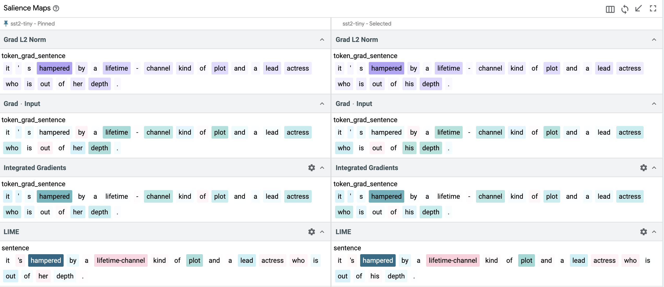
To gain some confidence in our heuristic, we look for examples where Grad · Input performs poorly compared to the other methods. There are quite a few in the dataset, for example the sentence below where Grad · Input predicts completely opposite salience scores to its counterparts.

An example of how Grad · Input can perform poorly—all pink values, the opposite of what. other methods found—on certain input and model architecture combinations.

Use Case 1: Sexism Analysis with Counterfactuals

Coming back to our use-case, we want to investigate if the model displays sexist behavior for a particular input sentence. We take a datapoint with a negative sentiment label, which talks about the performance of an actress in the movie.

The key words/tokens (based on salience scores across the three chosen methods) in this sentence are “hampered”, “lifetime-channel”, “lead”, “actress”, “her” and “depth”. The only words out of this which are related to gender are “actress” and “her”. The words “actress” and “her” get a significant weight for both Grad L2 Norm and IG, and is assigned a positive score (IG scores are slightly stronger than Grad L2 Norm scores), indicating that the gender of the person is helping the model be sure of its predictions of this sentence being a negative review sentiment. However for LIME, the salience scores for these two words is a small negative number, indicating that the gender of the model is actually causing a small decrease in model confidence for the prediction of this being a negative review. Even with this small disparity between the token-based and blackbox methods in the gender related words in the sentence, it turns out that these are not the most important words. “Hampered”, “lifetime-channel” and “plot” are the dominating words/tokens for this particular example in helping the model make its decision. We still want to explore if reversing the gender might change this. Would it make the model give more or less importance to other tokens or the tokens we replaced? Would it change the model prediction confidence scores?

To do this, we generate a counterfactual example using the Datapoint Editor which is located right beside the Data Table in the UI, changing "actress" with "actor" and "her" with "his" after selecting our datapoint of interest. An alternative to this approach is to use the Word replacer under the Counterfactuals tab in the bottom half of the LIT app to achieve the same task. If our model is predicting a negative sentiment due to sexist influences towards “actress” or “her”, then the hypothesis is that it should show opposite sentiments if we flip those key tokens.

Manually generating a counterfactual example in the Datapoint Editor, in this case changing "actress" to "actor" and "her" to "his", does not induce much change in the token salience scores.

However, it turns out that there is very minimal (and hence negligible) change in the salience score values of any of the tokens. The model doesn't change its prediction either. It still predicts this to be a negative review sentiment with approximately the same prediction confidence. This indicates that at least for this particular example, our model isn't displaying sexist behavior and is actually making its prediction based on key tokens in the sentence which are not related to the gender of the actress/actor.

Use Case 2: Pairwise Comparisons

Let's take another example. This time we consider the sentence “a sometimes tedious film” and generate three counterfactuals, first by replacing the two words “sometimes” and “tedious” with their respective antonyms one-by-one and then together to observe the changes in predictions and salience.

To create the counterfactuals, we can simply use the Datapoint Editor which is located right beside the Data Table in the UI. We can just select our data point of interest (data point 6), and then replace the words we are interested in with the respective substitutes. Then we assign a label to the newly created sentence and add it to our data. For this particular example, we are assigning 0 when "tedious" appears and 1 when "exciting" appears in the sentence. An alternative to this approach is to use the Word replacer under the Counterfactuals tab in the bottom half of the LIT app to achieve the same task.

The Data Table and Datapoint Editor modules showing the three manually generated counterfactuals that will be used to explore pairwise comparisons of salience results.

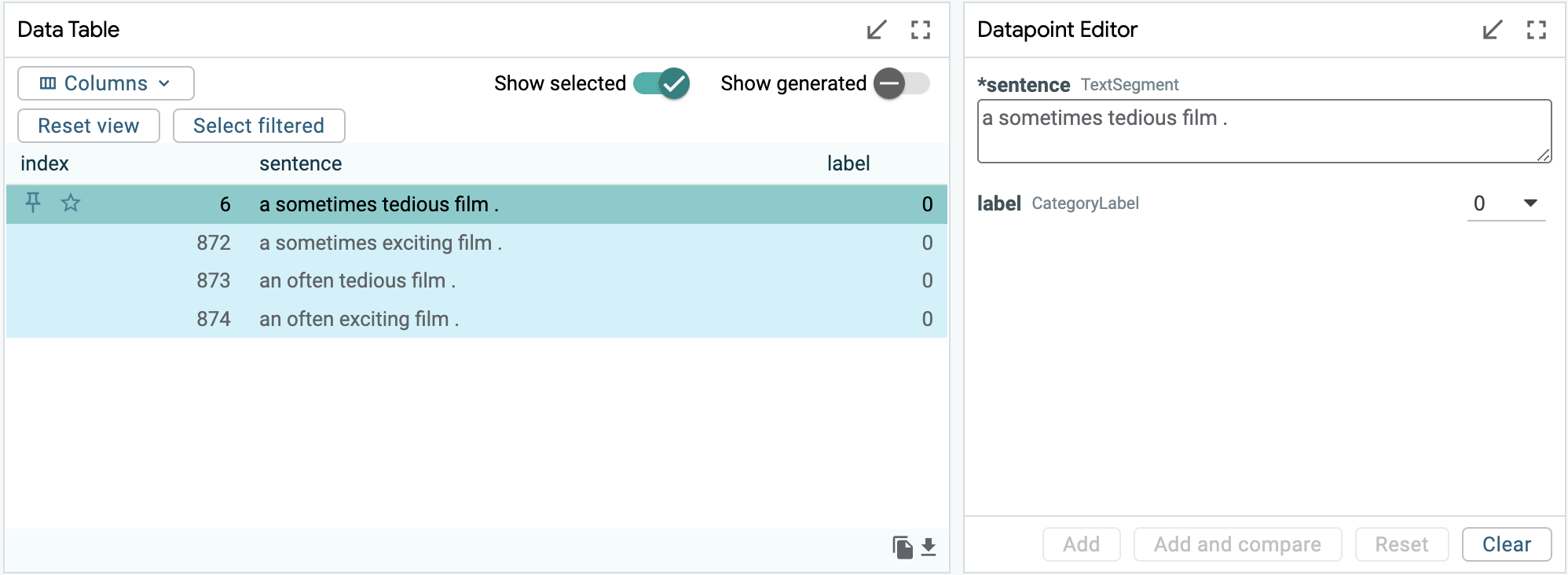
We can pin the original sentence in the data table and then cycle through the three available pairs by selecting each of the new sentences as our primary selection. This will give us a comparison-type output in the Salience Maps module between the pinned and the selected examples.

A table of the salience scores for each token in the inputs.

When we replace “sometimes” with “often”, it gets a negative score of almost equal magnitude (reversing polarity) from LIME which makes sense, because “often” makes the next word in the sentence more impactful, linguistically. The model prediction doesn't change either, and this new review is still classified as having a negative sentiment.

Replacing "sometimes" with "often" had a minimal impact on the gradient-based salience interpreters, but it did flip the polarity of that token in the LIME results.

On replacing “tedious” with “exciting”, the salience for “sometimes” changes from positive score to negative in the LIME output. In the IG output, “sometimes” changes from a strong positive score to a weak positive score. These changes are also justified because in this new sentence “sometimes” counters the positive effect of the word “exciting”. The main negative word in our original datapoint was “tedious” and by replacing this with a positive word “exciting”, the model's classification of this new sentence also changes and the new sentence is classified as positive with a very high confidence score.

Replacing "tedious" with "exciting" had a substantial impact on the salience interpreters that output signed results, but only a minimal impact on the Grad L2 Norm interpreter.

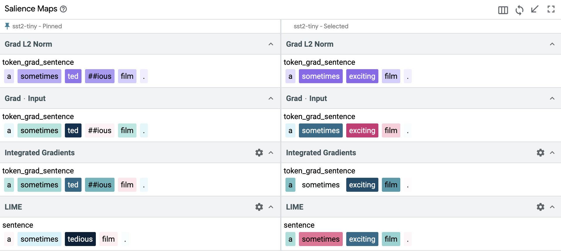
And finally, when we replace both “sometimes tedious” with “often exciting”, we get strong positive scores from both LIME and IG, which is in line with the overall strong positive sentiment of the sentence. The model predicts this new sentence as positive sentiment, and the confidence score for this prediction is slightly higher than the previous sentence where instead of “often” we had used “sometimes”. This makes sense as well because “often” enhances the positive sentiment slightly more than using “sometimes” in a positive review.

Replacing both "sometimes" and "tedious" has a substantial impact on all salience interpreters, attenuating some results, accentuating others, and in the case of Grad · Input, demonstrating how this counterfactual captures an opposing sentiment to the original.

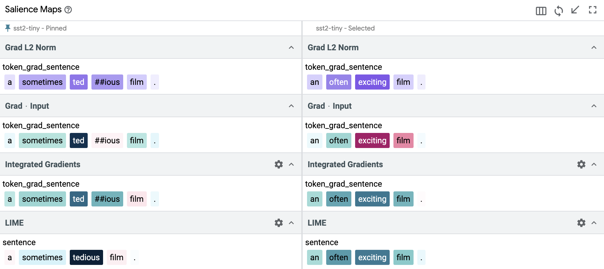
In this second example, we mostly based our observation on LIME and IG, because we could observe visual changes directly from the outputs of these methods. Grad L2 Norm outputs were comparatively inconclusive, highlighting the need to select appropriate methods and compare results between them. The model predictions were in line with our expected class labels and the confidence scores for predictions on the counterfactuals could be justified using salience scores assigned to the new tokens.

Use Case 3: Quality Assurance

A real life use case for the salience maps module can be in Quality Assurance. For example, if there is a failure in production (e.g., wrong results for a search query), we know the text input and the label the model predicted. We can use LIT Salience Maps to debug this failure and figure out which tokens were most influential in the prediction of the wrong label, and which alternative labels could have been predicted (i.e., is there one clear winner, or are there a few that are roughly the same?). Once we are done with debugging using LIT, we can make the necessary changes to the model or training data (eg. adding fail-safes or checks) to solve the production failure.

Conclusion

Three gradient-based salience methods and one black box method are provided out of the box to LIT users who need to use these post-hoc interpretations to make sense of their language model's predictions. This diverse array of built-in techniques can be used in combination with other LIT modules like counterfactuals to support robust exploration of a model's behavior, as illustrated in this tutorial. And as always, LIT strives to enable users to add their own salience interpreters to allow for a wider variety of use cases beyond these default capabilities!