Have you ever eaten a hot dog with hot sauce on a hot day? Even if you have not, you still understood the question—which is remarkable, since hot was used in three completely different senses. Humans effortlessly take context into account, disambiguating the multiple meanings.
Bringing this same skill to computers has been a longstanding open problem. A recently invented technique, the Transformer architecture, is designed in a way that may begin to address this challenge. Our paper explores one particular example of this type of architecture, a network called BERT.
One of the key tools for representing meaning is a "word embedding," that is, a map of words into points in high-dimensional Euclidean space. This kind of geometric representation can capture a surprisingly rich set of relationships between words, and word embeddings have become a critical component of many modern language-processing systems.
The catch is that traditional word embeddings only capture a kind of "average" meaning of any given word--they have no way to take context into account. Transformer architectures are designed to take in a series of words--encoded via context-free word embeddings--and, layer by layer, transform them into "context embeddings." The hope is that these context embeddings will somehow represent useful information about the usage of those words in the particular sentence they appear. In other words, in the input to BERT, the word hot would be represented by the same point in space, no matter whether it appears next to dog, sauce, or day. But in subsequent layers, each hot would occupy a different point in space.
In this blog, we describe visualizations that help us explore the geometry of these context embeddings--and which suggest that context embeddings do indeed capture different word senses. We then provide quantitative evidence for that hypothesis, showing that simple classifiers on context embedding data may be used to achieve state-of-the-art results on standard word sense disambiguation tasks. Finally, we show that there is strong evidence for a semantic subspace within the embedding space, similar to the syntactic subspace described by Hewitt and Manning, and discussed in the first post of this series.
So, which subtleties are captured in these embeddings, and which are lost? To understand this, we approach the question with a visualization which attempts to isolate the contextual information of a single word across many instances. How does BERT understand the meaning of a given word in each of these contexts?
When a word (e.g., hot)is entered, the system retrieves 1,000 sentences from wikipedia that contain hot. It sends these sentences to BERT as input, and for each one it retrieves the context embedding for hot at each layer.
The system then visualizes these 1,000 context embeddings using UMAP. The UMAP projection generally shows clear clusters relating to word senses, for example hot as in hot day or as in hot dog. Different senses of a word are typically spatially separated, and within the clusters there is often further structure related to fine shades of meaning.
To make it easier to interpret the visualization without mousing over every point, we added labels of words that are common between sentences in a cluster.
A natural question is whether the space is partitioned by part of speech. Showing the parts of speech can be enabled in the UI with the "show POS" toggle. The dots are then colored by the part of speech of the query word, and the labels are then uncolored.
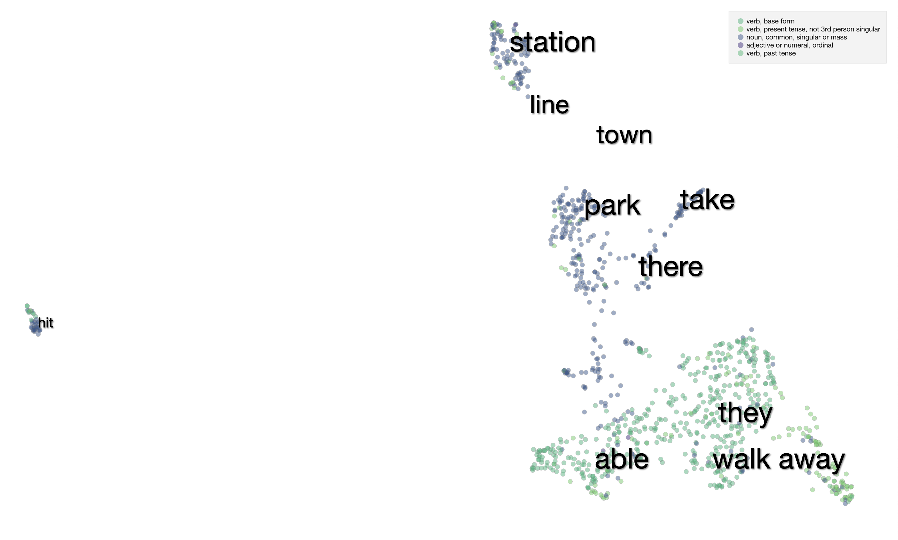
Indeed, this is the case. The words are partitioned into nouns and verbs.
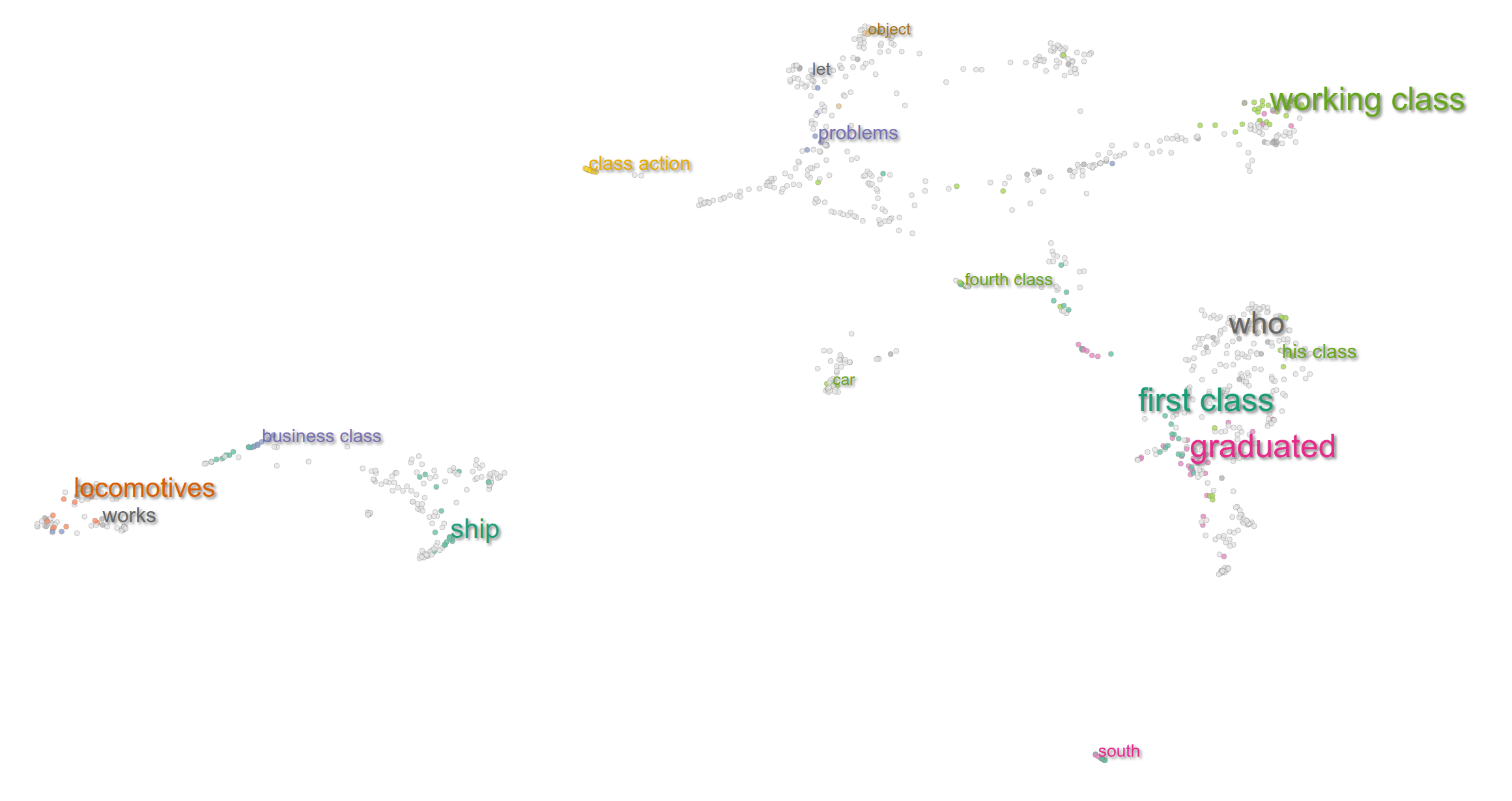
The separation of clusters goes beyond parts-of-speech. For the word class, below, the space is partitioned more subtly. To the top right, there is a cluster of sentences about working class, middle/upper/lower classes, etc. Below is the cluster for the educational sense of the word-- high school classes, students taking classes, etc. Still more clusters can be found for class-action lawsuits, equivalence classes in math, and more.
The previous examples have all used embeddings from the last layer of BERT. But where do these clusters arise, and what do the embeddings look like as they progress through the network?
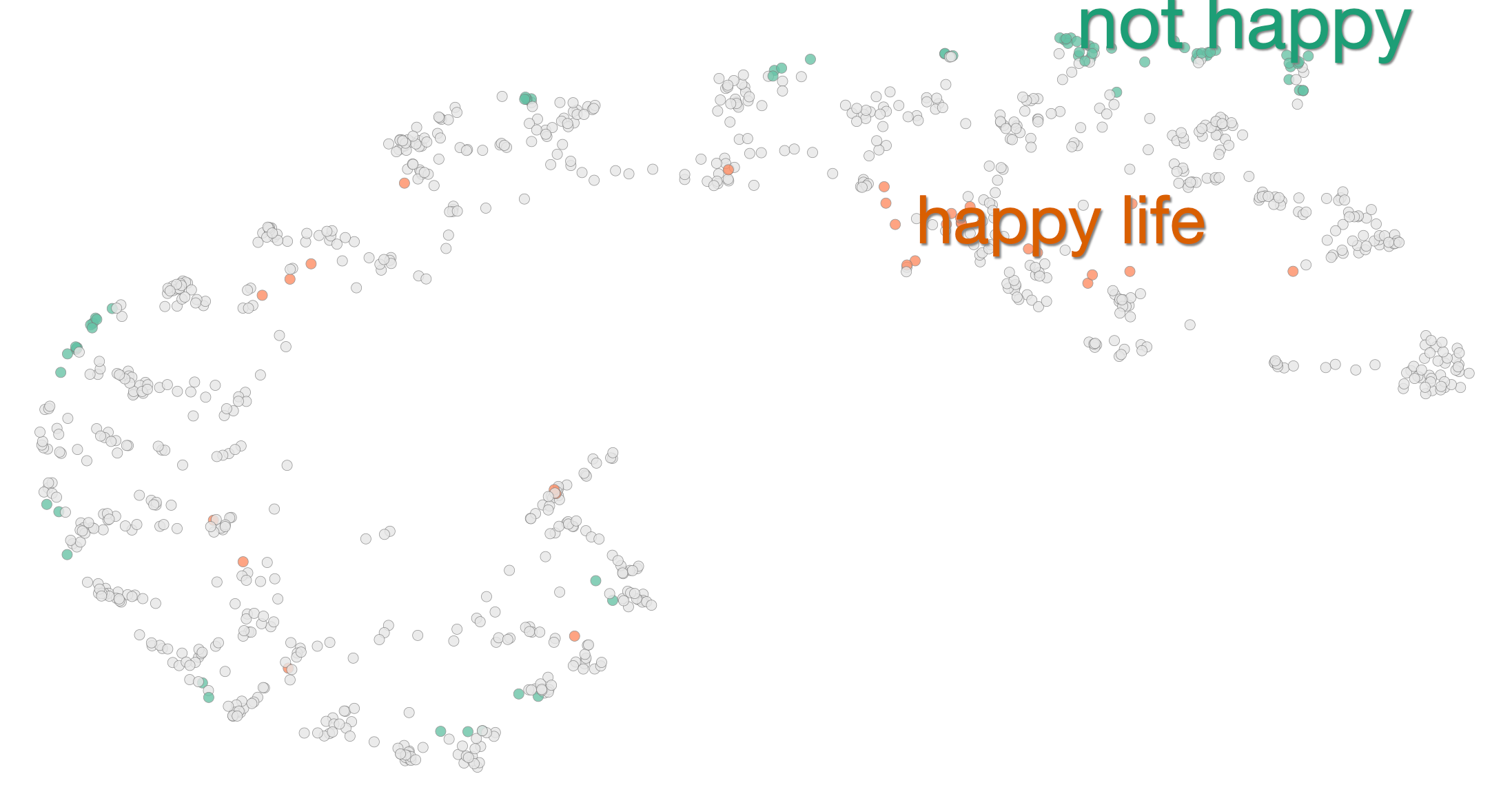
For most words that only have one sense (e.g., happy or man), the earliest layer (token embeddings + positional embeddings, with one transformer layer) has a canonical spiral pattern. This pattern turns out to be based on the position of the word in the sentence, and reflects the way linear order is encoded into the BERT input. For example, the sentences with happy as the third word are clustered together, and are between the sentences with happy as the second word, and those with happy as the fourth word.
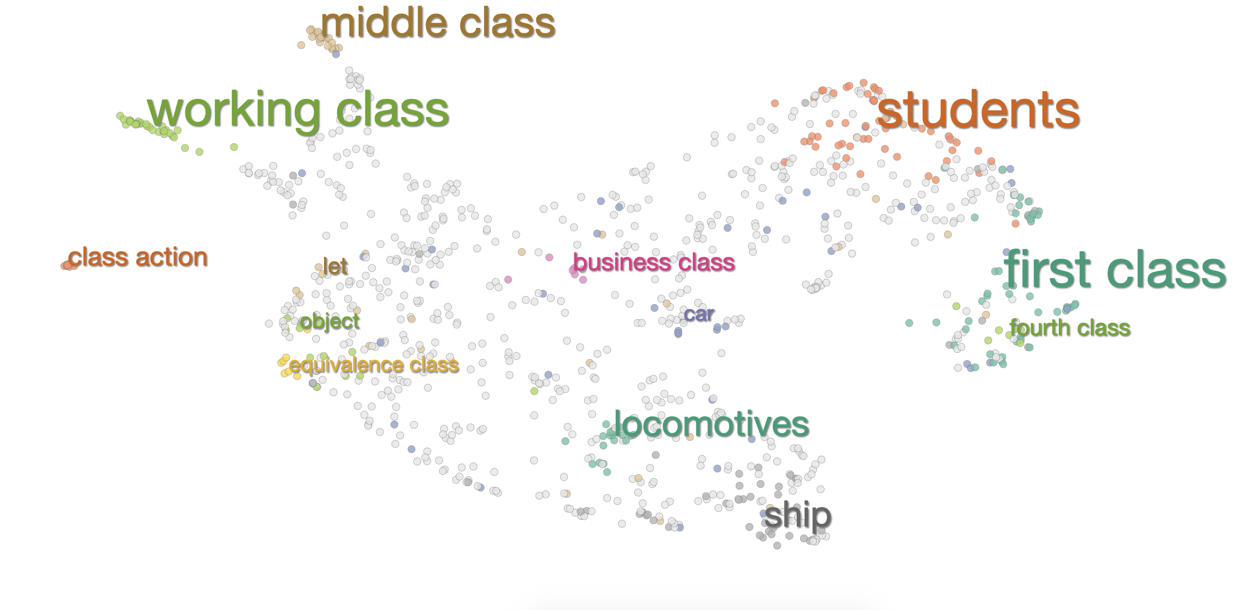
Interestingly, many words (e.g., civil, class, and state), do not have this pattern at the first layer. Below are the embeddings for class at the first layer, which are already semantically clustered.
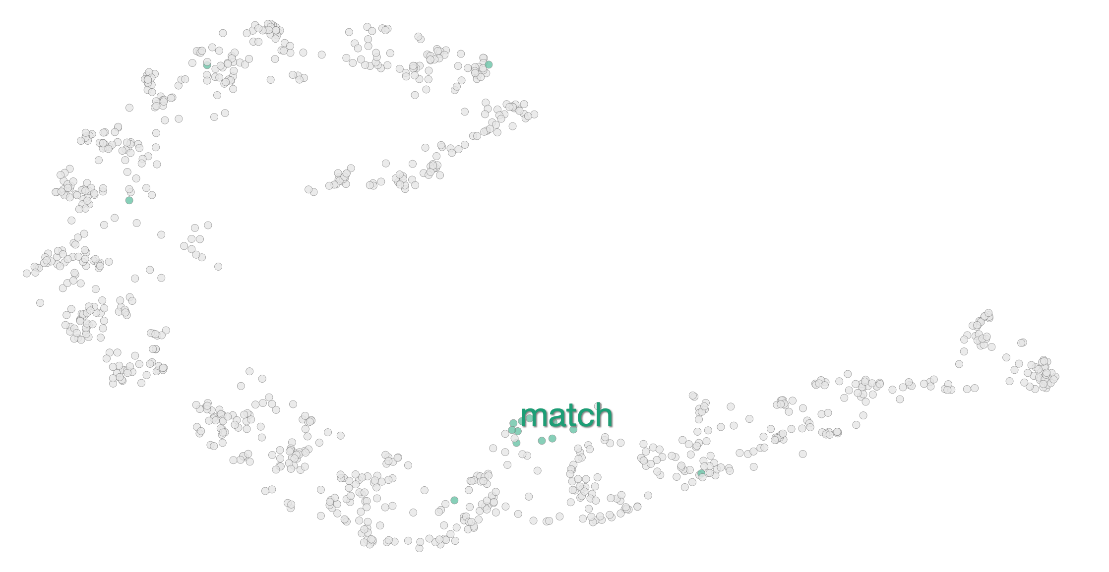
So what about the layers in between? Interestingly, there are often more disparate clusters in the middle of the model. The reason for this is somewhat of an open question. We know from Tenney et al that BERT performs better on some semantic and syntactic tasks with embeddings from the middle of the model. Perhaps there is some information that is lost towards the later layers in service of some higher level task, that causes the more merged cluster.
Another observation is that, towards the end of the network, most of the attention is paid to the CLS and SEP tokens (special tokens at the beginning and end of the sentence.) We’ve conjectured that this could make all clusters merge together to some degree.
The apparent detail in the clusters we visualized raises two immediate questions: first, can we quantitatively demonstrate that BERT embeddings capture word senses? Second, how can we resolve the fact that we observe BERT embeddings capturing semantics, when previously we saw those same embeddings capturing syntax?
The crisp clusters seen in the visualizations above suggest that BERT may create simple, effective internal representations of word senses, putting different meanings in different locations.
To test this out quantitatively, we trained a simple nearest-neighbor classifier on these embeddings to perform word sense disambiguation (WSD).
We follow the procedure described by Peters et al, who performed a similar experiment with the ELMo model. For a given word with n senses, we make a nearest-neighbor classifier where each neighbor is the centroid of a given word sense’s BERT-base embeddings in the training data. To classify a new word we find the closest of these centroids, defaulting to the most commonly used sense if the word was not present in the training data.
The simple nearest-neighbor classifier achieves an F1 score of 71.1, higher than the current state of the art, with the accuracy monotonically increasing through the layers. This is a strong signal that context embeddings are representing word-sense information. Additionally, we got an higher score of 71.5 using the technique described in the following section.
Hewitt and Manning found that there was an embedding subspace that appeared to contain syntactic information. We hypothesize that there might also exist a subspace for semantics. That is, a linear transformation under which words of the same sense would be closer together and words of different senses would be further apart.
To explore this hypothesis, we trained a probe following Hewitt and Manning’s methodology.
We initialized a random matrix $B\in{R}^{k\times m}$, testing different values for $m$. Loss is, roughly, defined as the difference between the average cosine similarity between embeddings of words with different senses, and that between embeddings of the same sense.
We evaluate our trained probes on the same dataset and WSD task used in part 2. As a control, we compare each trained probe against a random probe of the same shape. As mentioned, untransformed BERT embeddings achieve a state-of-the-art accuracy rate of 71.1%. We find that our trained probes are able to achieve slightly improved accuracy down to $m$ = 128 dimensions.
Though our probe achieves only a modest improvement in accuracy for final-layer embeddings, we note that we were able to more dramatically improve the performance of embeddings at earlier layers (see the Appendix in our paper for details: Figure 10). This suggests there is more semantic information in the geometry of earlier-layer embeddings than a first glance might reveal. Our results also support the idea that word sense information may be contained in a lower-dimensional space. This suggests a resolution to the question mentioned above: word embeddings encode both syntax and semantics, but perhaps in separate complementary subspaces.
Since embeddings produced by transformer models depend on context, it is natural to speculate that they capture the particular shade of meaning of a word as used in a particular sentence. (E.g., is bark an animal noise or part of a tree?) It is still somewhat mysterious how and where this happens, though. Through the explorations described above, we attempt to answer this question both qualitatively and quantitatively with evidence of geometric representations of word sense.
Many thanks to David Belanger, Tolga Bolukbasi, Dilip Krishnan, D. Sculley, Jasper Snoek, Ian Tenney, and John Hewitt for helpful feedback and discussions about this research. For more details, and results related to syntax as well as semantics, please read our full paper! And look for future notes in this series.