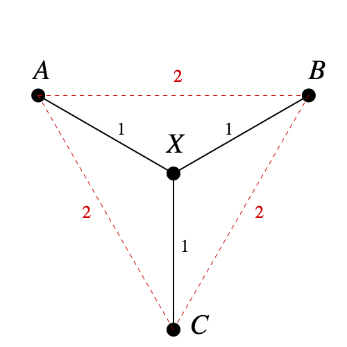
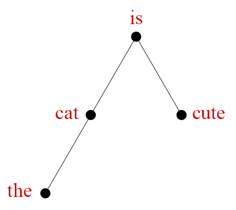
Figure 1. You can't isometrically embed this tree in Euclidean space.
Language is made of discrete structures, yet neural networks operate on continuous data: vectors in high-dimensional space. A successful language-processing network must translate this symbolic information into some kind of geometric representation—but in what form? Word embeddings provide two well-known examples: distance encodes semantic similarity, while certain directions correspond to polarities (e.g. male vs. female).
A recent, fascinating discovery points to an entirely new type of representation. One of the key pieces of linguistic information about a sentence is its syntactic structure. This structure can be represented as a tree whose nodes correspond to words of the sentence. Hewitt and Manning, in A structural probe for finding syntax in word representations, show that several language-processing networks construct geometric copies of such syntax trees. Words are given locations in a high-dimensional space, and (following a certain transformation) Euclidean distance between these locations maps to tree distance.
But an intriguing puzzle accompanies this discovery. The mapping between tree distance and Euclidean distance isn't linear. Instead, Hewitt and Manning found that tree distance corresponds to the square of Euclidean distance. They ask why squaring distance is necessary, and whether there are other possible mappings.
This note provides some potential answers to the puzzle. We show that from a mathematical point of view, squared-distance mappings of trees are particularly natural. Even certain randomized tree embeddings will obey an approximate squared-distance law. Moreover, just knowing the squared-distance relationship allows us to give a simple, explicit description of the overall shape of a tree embedding.
We complement these geometric arguments with analysis and visualizations of real-world embeddings in one network (BERT) and how they systematically differ from their mathematical idealizations. These empirical findings suggest new, quantitative ways to think about representations of syntax in neural networks. (If you're only here for empirical results and visualizations, skip right to that section.)
In fact, the tree in Figure 1 is one of the standard examples to show that not all metric spaces can be embedded in $\mathbb{R}^n$ isometrically. Since $d(A, B) = d(A, X) + d(X, B)$, in any embedding $A$, $X$, and $B$ will be collinear. The same logic says $A$, $X$, and $C$ will be collinear. But that means $B = C$, a contradiction.
If a tree has any branches at all, it contains a copy of this configuration, and can't be embedded isometrically either.
By contrast, squared-distance embeddings turn out to be much nicer—so nice that we'll give them a name. The reasons behind the name will soon become clear.
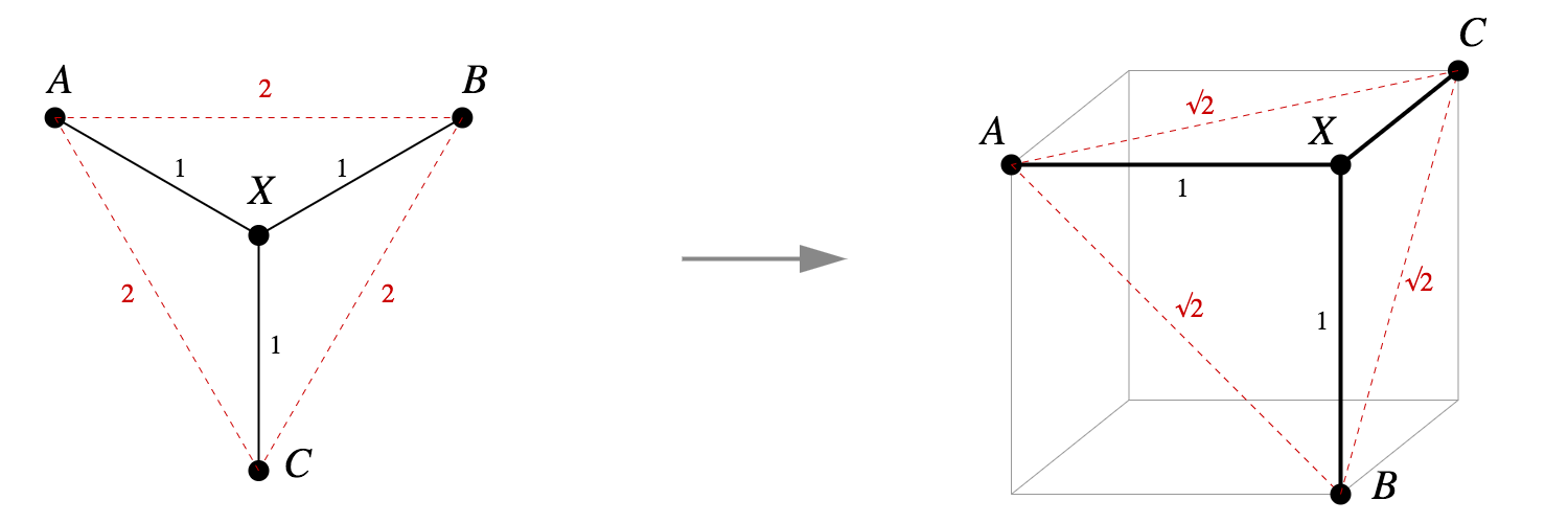
Does the tree in Figure 1 have a Pythagorean embedding? Yes: as seen in Figure 2, we can assign points to neighboring vertices of a unit cube, and the Pythagorean theorem gives us what we want.
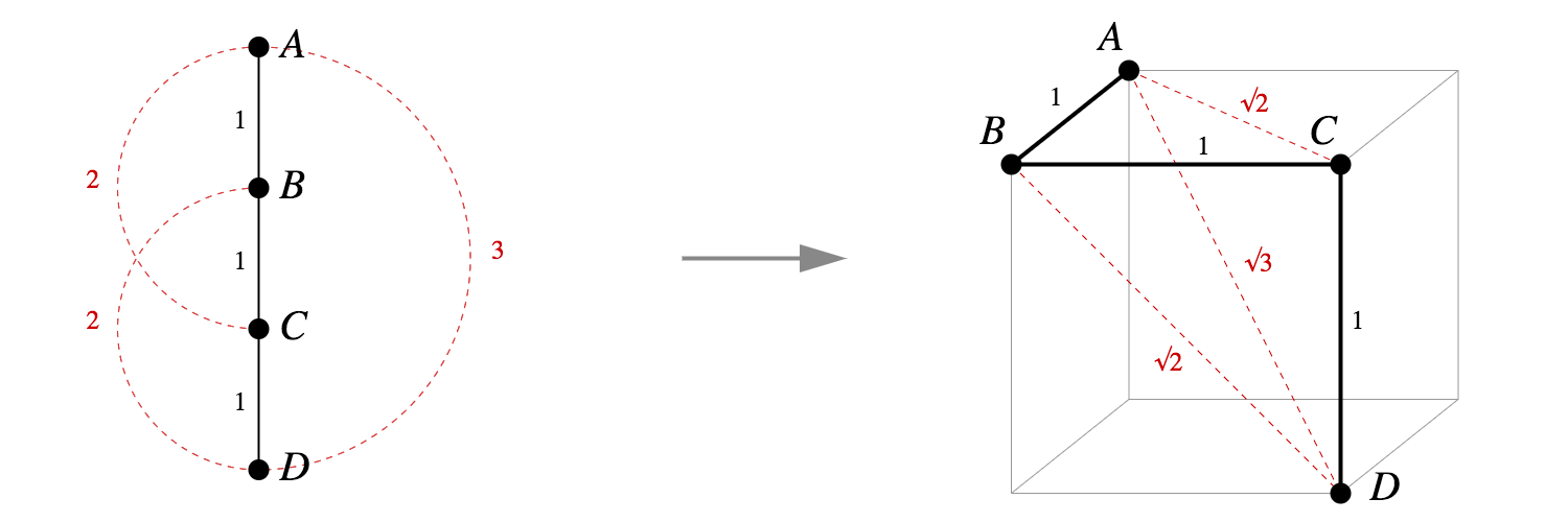
What about other small trees, like a chain of four vertices? That too has a tidy Pythagorean embedding into the vertices of a cube.
These two examples aren't flukes. It's actually straightforward to write down an explicit Pythagorean embedding for any tree into vertices of a unit hypercube.
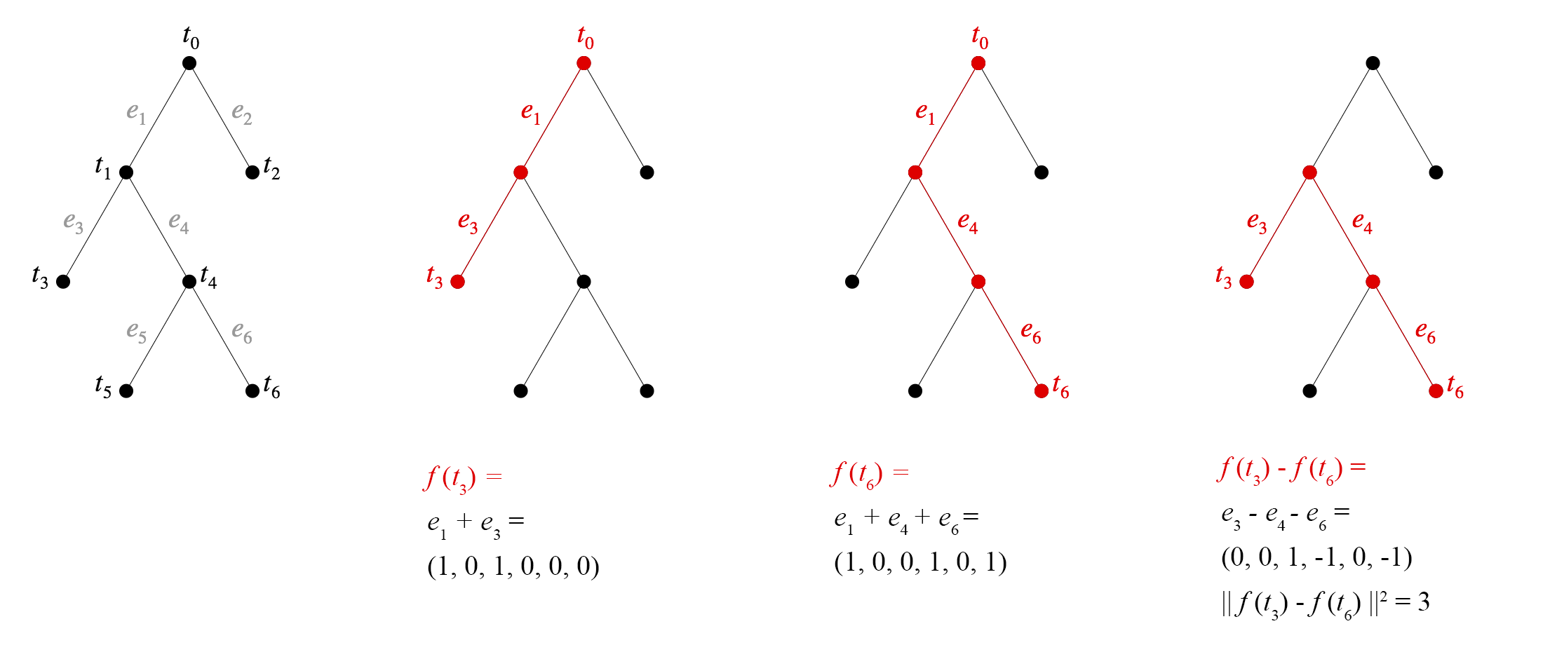
One way to view this construction is that we've assigned a basis vector to each edge. To figure out the embedding for a node, we walk back to the root and add up all the vectors for the edges we pass. See figure below.
The value of this proof is not just the existence result, but in the explicit geometric construction. Any two Pythagorean embeddings of the same tree are isometric—and related by a rotation or reflection—since distances between all pairs of points are the same in both. So we may speak of the Pythagorean embedding of a tree, and this theorem tells us exactly what it looks like.
Moreover, the embedding in Theorem 1.1 has a clean informal description: at each embedded vertex of the graph, all line segments to neighboring vertices are unit-distance segments, orthogonal to each other and to every other edge segment. If you look at Figures 1 and 2, you'll see they fit this description.
It's also easy to see the specific embedding constructed in the proof is a tree isometry in the $\ell^1$ metric, although this depends strongly on the axis alignment.
We can make a slight generalization of Theorem 1.1. Consider trees where edges have weights, and the distance between two nodes is the sum of weights of the edges on the shortest path between them. In this case, too, we can always create a Pythagorean embedding.
The embedding in Theorem 1.2, despite being axis-aligned, is no longer an isometry with respect to the $\ell^1$ metric. However, if we use vectors $w_i e_i$ rather than ${w_i}^{1/2} e_i$ we can recover an $\ell^1$ isometry.
On the other hand, it turns out that power-$p$ tree embeddings will not necessarily even exist when $p < 2$.
See our paper for a proof (and an alternative proof may be found here). To summarize the idea, for any given $p < 2$, there is not enough “room” to embed a node with sufficiently many children.
The Pythagorean embedding property is surprisingly robust, at least in spaces whose dimension is much larger than the size of the tree. (This is the case in our motivating example of language-processing neural networks, for instance.) In the proofs above, instead of using the basis $e_1, \ldots, e_{n-1} \in \mathbb{R}^{n-1}$ we could have chosen $n$ vectors completely at random from a unit Gaussian distribution in $\mathbb{R}^{m}$. If $m \gg n$, with high probability the result would be an approximate Pythagorean embedding.
The reason is that in high dimensions, (1) vectors drawn from a unit Gaussian distribution have length very close to 1 with high probability; and (2) when $m \gg n$, a set of $n$ unit Gaussian vectors will likely be close to mutually orthogonal.
In other words, in a space that is sufficiently high-dimensional, a randomly branching embedding of a tree, where each child is offset from its parent by a random unit Gaussian vector, will be approximately Pythagorean.
This construction could even be done by an iterative process, requiring only “local” information. Initialize with a completely random tree embedding, and in addition pick a special random vector for each vertex; then at each step, move each child node so that it is closer to its parent's location plus the child's special vector. The result will be an approximate Pythagorean embedding.
The simplicity of Pythagorean embeddings, as well as the fact that they arise from a localized random model, suggests they may be generally useful for representing trees. With the caveat that tree size is controlled by the ambient dimension, they may be a low-tech alternative to approaches based on hyperbolic geometry.
We won't describe the BERT architecture here, but roughly speaking the network takes as input a sequences of words, and across a series of layers produces a series of embeddings for each of these words. Because these embeddings take context into account, they're often referred to as context embeddings.
There is one twist: first you need to transform the context embeddings by a certain matrix $B$, a so-called structural probe. But following that, the square of the Euclidean distance between two words' context embeddings approximates the parse tree distance between the two words.
Here is where the math in the previous section pays off. In our terminology, the context embeddings approximate a Pythagorean embedding of a sentence's dependency parse tree. That means we have a good idea—simply from the squared-distance property and Theorem 1.1—of the overall shape of the tree embedding.
We then project these points to two dimensions via PCA. To show the underlying tree structure, we connect pairs of points representing words that have a dependency relation. Figure 5, below, shows the result for a sample sentence and, for comparison, PCA projections for the same data of an exact Pythagorean embedding; randomly branched embeddings; and embeddings where node coordinates are completely random.
The PCA projection is already interesting—there's a definite resemblance between the BERT embedding and the idealization. Figure 5c shows a series of randomly branching embeddings, which also resemble the BERT embedding. As a baseline, Figure 5d shows a series of embeddings where words are placed independently at random.
But we can go one step further, and show how the embedding differs from an idealized model. In Figure 6 below, the color of each edge indicates the difference between Euclidean distance and tree distance. We also connect, with a dotted line, pairs of words without a dependency relation but whose positions (before PCA) were much closer than expected.
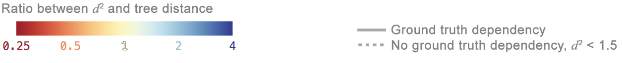
The resulting image lets us see both the overall shape of the tree embedding, and fine-grained information on deviation from a true Pythagorean embedding. Figure 5 shows two examples. These are typical cases, illustrating some common themes. In the diagrams, orange dotted lines connect part/of, same/as, and sale/of. This effect is characteristic, with prepositions are embedded unexpectedly close to words they relate to. We also see connections between two nouns showing up as blue, indicating they are farther apart than expected—another common pattern.
Figure 8, at the end of this article, shows additional examples of these visualizations, where you can look for further patterns.
Based on these observations, we decided to make a more systematic study of how different dependency relations might affect embedding distance. One way to answer this question is to consider a large set of sentences and test whether the average distance between pairs of words has any correlation with their syntactic relation.We performed this experiment with a set of Penn Treebank sentences, along with derived parse trees.
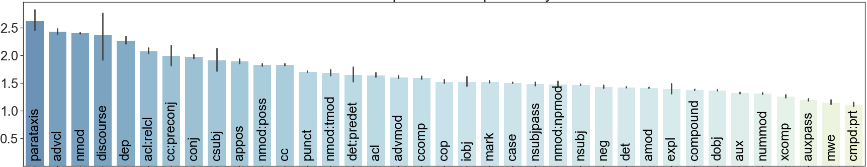
Figure 7 shows the results of this experiment. It turns out the average embedding distances of each dependency relation vary widely: from around 1.2 (compound : prt, advcl) to 2.5 (mwe, parataxis, auxpass). It is interesting to speculate on what these systematic differences mean. They might be the effects of non-syntactic features, such as word distance within a sentence. Or perhaps BERT’s syntactic representations have additional quantitative aspects beyond plain dependency grammar, using weighted trees.
Many thanks to James Wexler for help with this note. And thanks to David Belanger, Tolga Bolukbasi, Dilip Krishnan, D. Sculley, Jasper Snoek, and Ian Tenney for helpful feedback and discussions about this research. For more details, and results related to semantics as well as syntax, please read our full paper! And look for future notes in this series.